2021/4/24: 解决(?)公式渲染问题,卸了重装了渲染器,然后参考配置了服务器渲染
空间&频率域滤波
用于记录学习数字图像处理的历程(不完全同步学校课程,不定期摸鱼)
空间域滤波
直方图均衡化
直方图的形状往往与图像的外观有关。
- 在暗图像的直方图中,大多数直方图容器集中在灰度级较低的一端(靠近 0)
- 亮的图像的直方图中,多数直方图容器集中在灰度级的高端
- 低对比度的图像的直方图中,直方图容器基本位于灰度级的中间
- 高对比度图像的直方图,容器覆盖了较宽的范围,并且像素的分布是基本均匀的
直方图均衡化的数学原理我们暂且不提,假如我们把直方图每个部分出现频率和总统计量做除法,得到一个概率分布函数 ,均衡化变换就是将一个概率分布不规则,不均匀的变化为分布均匀的新的函数
 。
。
Python 代码
1
2
3
4
5
6
7
8
9
10
11
12
13
14
15
16
17
18
19
20
21
22
23
24
25
26
27
28
29
30
31
| from PIL import Image
import matplotlib.pyplot as plt
import numpy as np
img = Image.open("./IMG_2546.JPG").convert("L")
img_array = np.array(img)
x_num, y_num = img.size
plt.subplot(121)
plt.xticks([])
plt.yticks([])
plt.hist(img_array.flatten(), 256)
im_hist, bins = np.histogram(img_array.flatten(), 256, density=True)
cdf = im_hist.cumsum()
cdf = 255 * (cdf / cdf[-1])
img_array_transformed = np.interp(img_array.flatten(), bins[:256], cdf)
plt.subplot(122)
plt.hist(img_array_transformed, 256)
plt.xticks([])
plt.yticks([])
plt.savefig("exp.png")
plt.show()
|
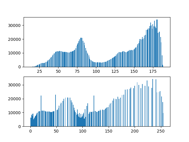
原直方图和均衡化后的图片的直方图:
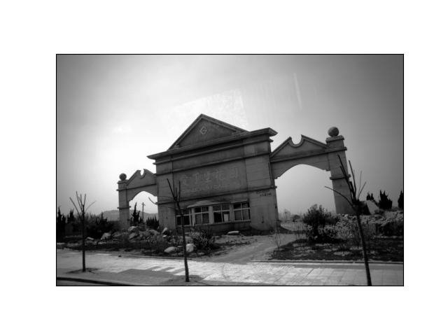
原图和均衡化后的图的对比:

如果我们对局部直方图均衡化,还可以显示出全局直方图均衡化无法显示的灰度细节。
低通空间滤波器
有现成的库可以调用:
1
2
| from PIL import Image, ImageFilter
img = img.filter(ImageFilter.GaussianBlur(radius=2))
|
高通空间滤波器
1
2
3
4
5
6
7
8
9
10
11
12
13
14
15
| from scipy import signal
def sharpening_f(img_array, kernel, c):
new_array = signal.convolve2d(img_array, kernel,
boundary='symm',
mode='same')
new_array[new_array > 255] = 255
new_array[new_array < 0] = 0
new_array = img_array + c*new_array
new_array[new_array > 255] = 255
new_array[new_array < 0] = 0
return new_array
|
横方向的 Sobel 算子,用于提取出水平方向的边界:

拉普拉斯是导数算子,因此会突出图像中急剧的灰度过渡,并不强调缓慢变化的灰度区域,这会使得原图像产生灰色边缘线和其他不连续的特征,因此将原图像与拉普拉斯变换后的图像相加就能够恢复背景特征,并且保留拉普拉斯锐化的效果。
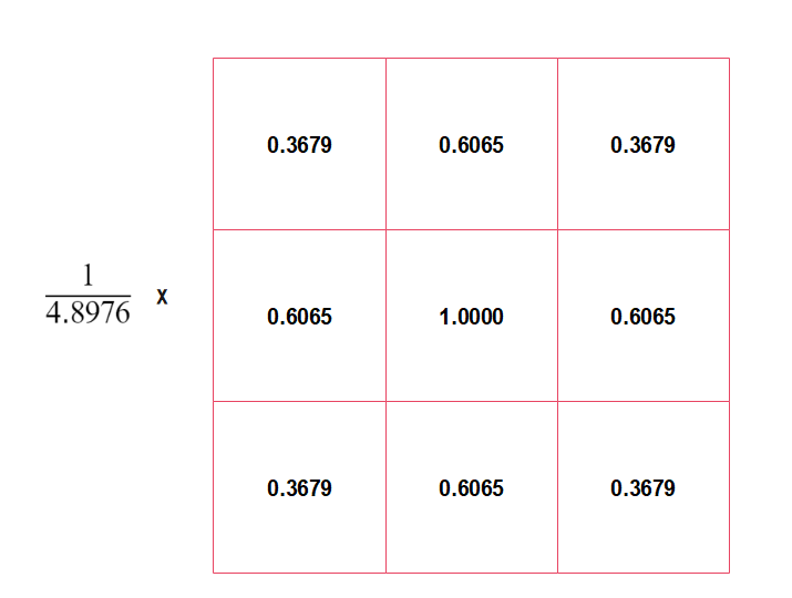
一种拉普拉斯核如下:

又或者是:

分为三个步骤:
- 模糊原图像
- 从原图中减去模糊后的图像(产生的差称为模板)
- 将模板与原图像相加
令  表示模糊后的图像,钝化掩蔽的过程可以用公式表示为:
%20-%20%5Cbar%7Bf%7D(x%2C%20y)%20%20%5C%5C%20%0Ag(x%2C%20y)%20%3D%20f(x%2C%20y)%2Bkg_%7Bmask%7D(x%2C%20y)%0A%5Cend%7Bmatrix%7D%5Cright.%0A)
1
2
3
4
5
6
7
8
9
10
11
12
13
14
15
16
17
18
19
| from PIL import Image, ImageFilter
import numpy as np
import matplotlib.pyplot as plt
image = Image.open("./IMG_2546.JPG").convert("L")
origin_array = np.array(image)
blurred_image = image.filter(ImageFilter.BLUR)
blurred_array = np.array(blurred_image)
mask_array = origin_array - blurred_array
weight_k = 2
new_array = origin_array + weight_k * mask_array
fig, (ax1, ax2) = plt.subplots(1, 2)
ax1.hist(origin_array.flatten(), 256)
ax1.set_title("Origin")
ax2.hist(new_array.flatten(), 256)
ax2.set_title("shielding Sharpened")
plt.savefig("exp6_sharping2.png")
plt.show()
|
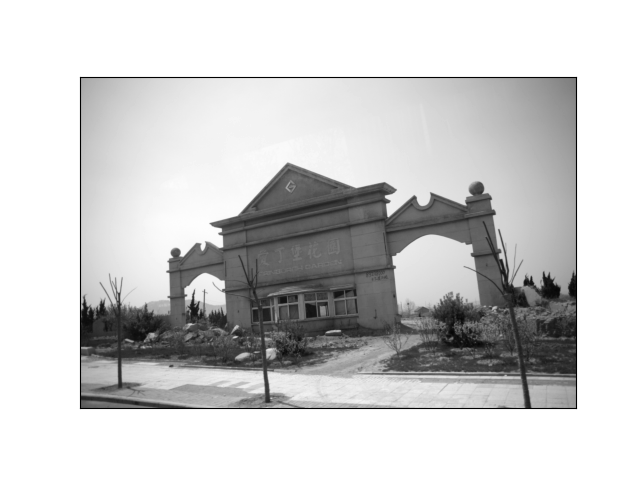
原图像:
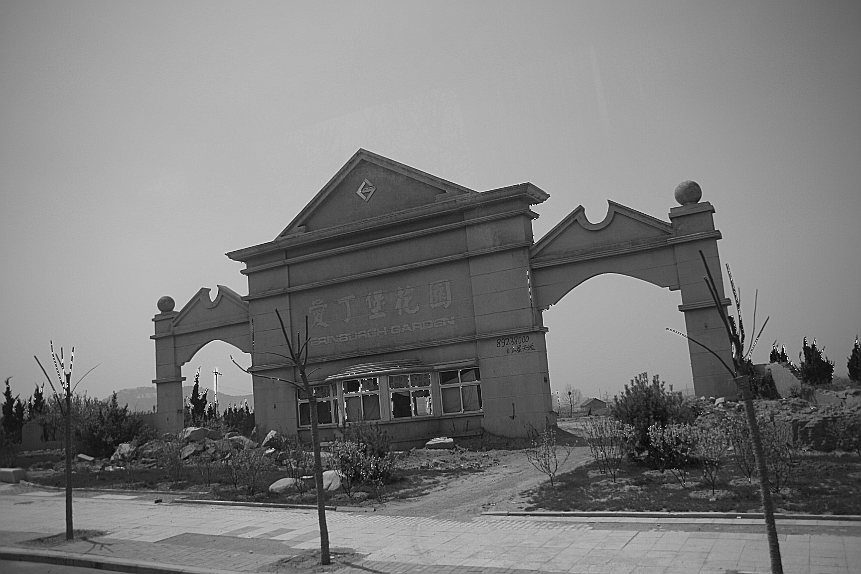
增强后的图像:
可以看到,我们仅仅是把 k 设置为 2,就出现了边界线。当  称为钝化掩蔽,
 时被称为高提升滤波,选择
  可以减少钝化模板的贡献。
频率域滤波
在深度学习出来前,频率域滤波一直是数字图像处理的比较热门的研究点(我们老师说的),频率域滤波的功能还是挺强大的,同样关于原理不过多介绍。
FFT&频谱
1
2
3
4
5
6
7
8
9
10
11
12
13
14
15
16
17
18
19
20
21
22
23
24
25
26
27
28
29
30
31
32
33
34
35
36
37
| import matplotlib.pyplot as plt
import numpy as np
import os
from PIL import Image
def fft_transform(in_path, name, out_path="."):
image = Image.open(in_path)
plt.subplot(221)
plt.imshow(image)
plt.axis("off")
plt.title("Origin Image")
image = image.convert("L")
plt.subplot(222)
plt.imshow(image, "gray")
plt.axis("off")
plt.title("Gray Image")
fft2 = np.fft.fft2(image)
log_fft2 = np.log(1 + np.abs(fft2))
shift2center = np.fft.fftshift(fft2)
log_shift2center = np.log(1 + np.abs(shift2center))
plt.subplot(223)
plt.imshow(np.absolute(shift2center), "gray")
plt.axis("off")
plt.title("shift2center")
plt.subplot(224)
plt.imshow(log_shift2center, "gray")
plt.axis("off")
plt.title("log_shift2center")
plt.savefig(os.path.join(out_path, ("fft_transformed_" + name)))
plt.clf()
|
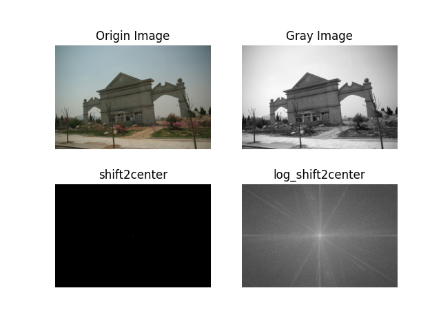
需要注意的是要对变换后的图像取 log,不然值太大会无法在正常的灰度级下显示。
高低通滤波器
课本上介绍的 3 个高通滤波器:
%5Cle%20D_0%5C%5C%0A%201%2C%20%26%20D(u%2Cv)%5Cgt%20D_0%0A%5Cend%7Bmatrix%7D%5Cright.%0A)
%2F2D_0%5E2%7D%0A)
%20%5Cright%20%5D%5E%7B2n%7D%7D%0A)
其中  表示截止频率到矩阵中心的距离,
 表示频率矩阵中心到矩阵中任意一点的距离。
1
2
3
4
5
6
7
8
9
10
11
12
13
14
15
16
17
18
19
20
21
22
23
24
25
26
27
28
29
30
31
32
33
34
35
36
37
38
39
40
41
42
43
44
45
46
47
48
49
50
51
52
53
54
55
56
57
58
59
60
61
62
63
64
65
66
67
68
| from PIL import Image
import numpy as np
import matplotlib.pyplot as plt
def cal_distance(pa, pb):
from math import sqrt
dis = sqrt((pa[0] - pb[0]) ** 2 + (pa[1] - pb[1]) ** 2)
return dis
class Filter:
@classmethod
def generate_filter(cls, d, shape, *args, **kwargs):
transfer_matrix = np.zeros(shape)
center_point = tuple(map(lambda x: (x - 1) // 2, shape))
for i in range(transfer_matrix.shape[0]):
for j in range(transfer_matrix.shape[1]):
dist = cal_distance(center_point, (i, j))
transfer_matrix[i, j] = cls.get_one(d, dist, *args, **kwargs)
return transfer_matrix
@classmethod
def get_one(cls, d, dist, *args, **kwargs) -> float:
return 1
class ILPFLowPassFilter(Filter):
@classmethod
def get_one(cls, d, dist, *args, **kwargs) -> float:
if dist <= d:
return 1
else:
return 0
class ILPFHighPassFilter(Filter):
@classmethod
def get_one(cls, d, dist, *args, **kwargs) -> float:
if dist <= d:
return 0
else:
return 1
class GaussianHighPassFilter(Filter):
@classmethod
def get_one(cls, d, dist, *args, **kwargs) -> float:
return 1 - np.exp(-(dist ** 2) / (2 * (d ** 2)))
class GaussianLowPassFilter(Filter):
@classmethod
def get_one(cls, d, dist, *args, **kwargs) -> float:
return np.exp(-(dist ** 2) / (2 * (d ** 2)))
class ButterworthFilter(Filter):
@classmethod
def get_one(cls, d, dist, *args, **kwargs) -> float:
n = kwargs["n"]
return 1 / ((1 + dist / d) ** (2 * n))
|
使用滤波器进行滤波:
1
2
3
4
5
6
7
8
9
10
11
12
13
14
15
16
|
choice = "material/1.jpg"
img = Image.open(choice).convert("L")
sq = min(img.size[0], img.size[1])
img = img.resize((sq, sq))
f = np.fft.fft2(img)
f_shift = np.fft.fftshift(f)
butter_filter_matrix = ButterworthFilter.generate_filter(30, img.size, n=2)
filter_matrix = np.fft.ifftshift(f_shift*butter_filter_matrix)
transform_img = np.abs(np.fft.ifft2(filter_matrix))
plt.axis("off")
plt.imshow(transform_img, cmap="gray")
plt.savefig("gauss_filter.png")
plt.show()
|
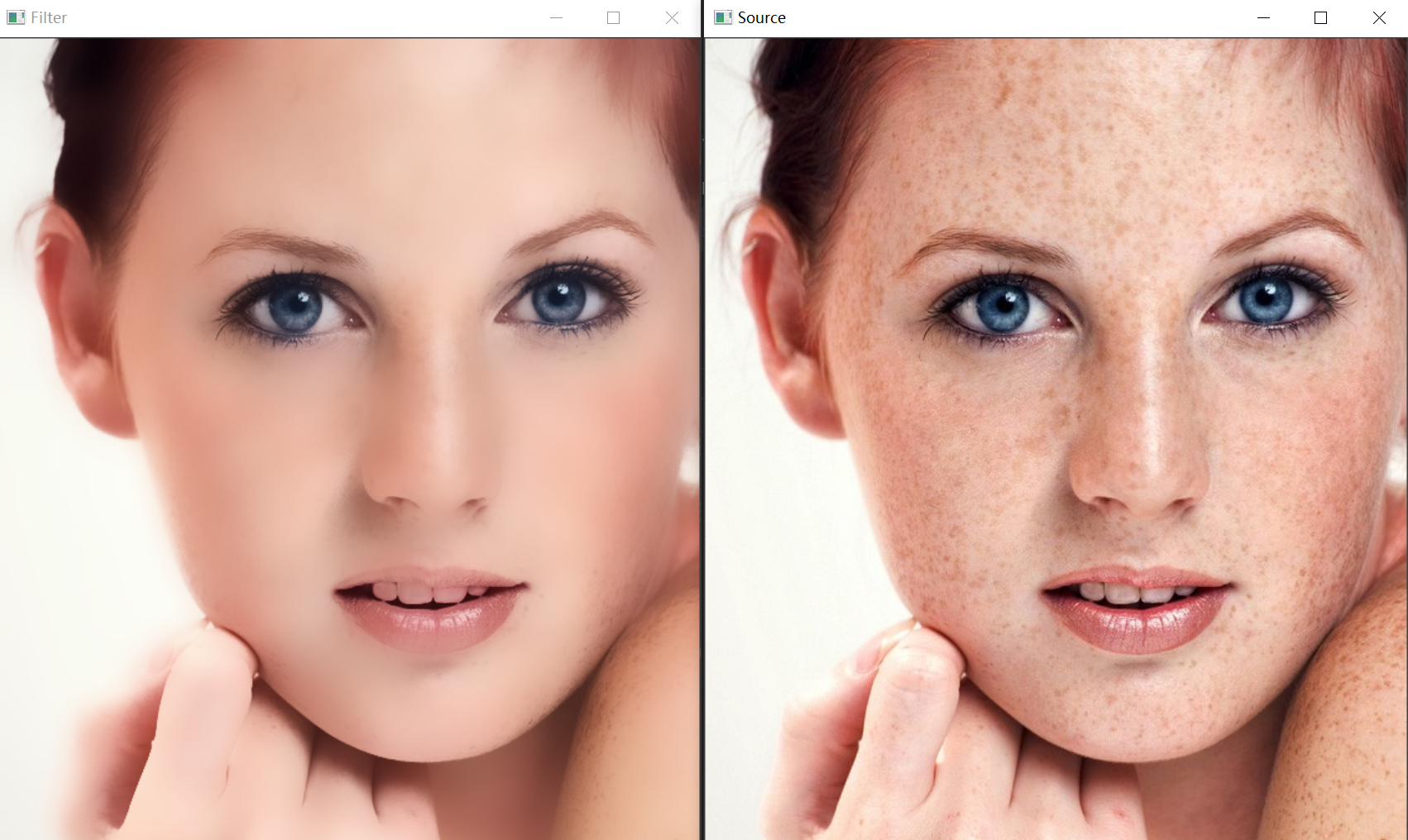
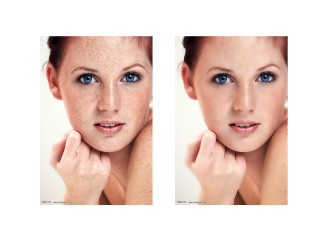
扩展:人脸磨皮算法
Bilateral
双边滤波(Bilateral filter)结合图像的空间邻近度和像素值相似度,同时考虑空域信息和灰度相似性,达到保边去噪的目的。
它的滤波器核由两个函数生成:空间域核和值域核。
空间域核是由像素位置欧式距离决定的模板权值,公式:
%5E2%2B(i-l)%5E2%7D%7B2%5Cdelta_d%5E2%7D)%0A)
其中i,j 代表的是当前坐标点的位置 k,l 为中心坐标点, 代表高斯函数的标准差。很明显
  是计算临近点 ij 到中心点的临近程度,因此空间域核是用于衡量空间临近的程度。这代表空间域的高斯函数。
值域核是由灰度像素值的差值决定模板的权值的:
-f(k%2Cl))%5E2%7D%7B2%5Cdelta_r%5E2%7D)%0A)
 代表每个点的灰度像素值,
 代表中点的像素值,
 也是值域核下高斯函数的标准差。将两者相乘就能得到双边滤波的模板权值:
*w_r(i%2Cj%2Ck%2Cl)%0A%3Dexp(-%5Cfrac%7B(i-k)%5E2%2B(i-l)%5E2%7D%7B2%5Cdelta_d%5E2%7D-%5Cfrac%7B(f(i%2Cj)-f(k%2Cl))%5E2%7D%7B2%5Cdelta_r%5E2%7D)%20%0A)
化简:
w(i%2Cj%2Ck%2Cl)%7D%7B%5Csum_%7Bkl%7Dw(i%2Cj%2Ck%2Cl)%7D%0A)
1
2
3
4
5
6
7
8
9
10
11
|
import cv2
file_name = './material/4.jpg'
image = cv2.imread(file_name)
dst = cv2.bilateralFilter(src=image, d=0, sigmaColor=100, sigmaSpace=15)
cv2.imshow("Source", image)
cv2.imshow("Filter", dst)
cv2.waitKey(0)
cv2.destroyAllWindows()
|
表面模糊
图像的表面模糊处理,其作用是在保留图像边缘的情况下,对图像的表面进行模糊处理。在对人物皮肤处理上,比高斯模糊更有效。(高斯模糊在使人物皮肤光洁的同时,也将一些边缘特征给模糊了)
在处理手法上,表面模糊也与前面提到的卷积处理手段不同,表面模糊是每一个像素点都有自己的卷积矩阵,而且还是 3 套,用以对应于像素的 R、G、B 分量。
表面模糊有 2 个参数,即模糊半径 r 和模糊阈值 T,模糊半径确定模糊的范围,而模糊范围确定的是卷积矩阵的大小,模糊矩阵是一个长宽相等的矩阵,长度  。
。
矩阵的中间元素是当前的像素点,其余的元素按照下面的方法计算:

 是图像值,
是图像值, 是模板矩阵中心的图像值
一般来说,会有预处理: 
根据卷积运算,每个像素通过表面模糊之后的值为:

1
2
3
4
5
6
7
8
9
10
11
12
13
14
15
16
17
18
19
20
21
22
23
24
25
26
27
28
29
30
31
32
33
34
35
36
37
38
39
40
41
|
import matplotlib.pyplot as plt
import numpy
from skimage import io
def sur_blur(origin, threshold, r):
transformed = origin * 1.0
row, col = origin.shape
w_size = r * 2 + 1
for i in range(r, row - 1 - r):
for j in range(r, col - 1 - r):
iij = origin[i-r: i+r+1, j-r: j+r+1]
i0 = numpy.ones([w_size, w_size]) * origin[i, j]
wij = 1 - abs(iij - i0) / (2.5 * threshold)
wij[wij < 0] = 0
tmp = iij * wij
transformed[i, j] = tmp.sum() / wij.sum()
return transformed
file_name = './material/4.jpg'
img = io.imread(file_name)
img_out = img * 1.0
boundary = 20
half_size = 10
img_out[:, :, 0] = sur_blur(img[:, :, 0], boundary, half_size)
img_out[:, :, 1] = sur_blur(img[:, :, 1], boundary, half_size)
img_out[:, :, 2] = sur_blur(img[:, :, 2], boundary, half_size)
img_out = img_out / 255
plt.subplot(121)
plt.imshow(img)
plt.axis('off')
plt.subplot(122)
plt.imshow(img_out)
plt.axis('off')
plt.savefig("surface_blur.png")
plt.show()
|
效果挺好,就是算的有点慢:
参考链接